A little Python script to convert your Landsat scenes to KEA format

Downloading all this Mars data is starting to fill up my hard disks, so one thing I decided to do was compress all the various Landsat images I have.

Here is a Python script that will convert all GeoTIFF files in the current directory to the KEA format, and create a new header for each *MTL.txt Landsat header that exists in the directory to refer to the .kea files, for the use of a program such as ARCSI.

Download link (Dropbox)

# David Trethewey 20-06-2014
#
# convert all .tif or .TIF files
# in the current directory to .kea files
# using GDAL
# Does not delete any TIF files
#
# Assumptions:
# the TIF files are in the current directory
# that this script is being run from
# GDAL is available with KEA support
# 
# Modifies any Landsat header *MTL.txt files so that
# arcsi.py works if you have compressed the
# band .TIF files to .kea
# Does not overwrite original header
#
# imports
import os.path
import sys

def replaceGTIFF_kea(inputtext):
    outputtext = ""   
    for w in inputtext:
        w = w.replace("GEOTIFF","KEA")
        w = w.replace(".TIF",".kea")
        # this line should be unnecessary since Landsat MTL files use capital letters      
        # but just in case you have one that doesn't
        w = w.replace(".tif",".kea")
        outputtext += w
    return outputtext

# find all *.TIF files and *MTL.txt files in the current directory
directory = os.getcwd()
dirFileList = os.listdir(directory)
# print dirFileList
tifFileList = [f for f in dirFileList if ((f[-4:]=='.TIF')or(f[-4:]=='.tif'))]
MTLFileList = [f for f in dirFileList if (f[-7:]=='MTL.txt')]

#output format (GDAL code)
outFormat = 'KEA'

# run gdal_translate on all TIFs to convert to KEA
for t in tifFileList:
    gdaltranscmd = "gdal_translate -of "+outFormat+" "+t+" "+t[:-4]+".kea"
    print gdaltranscmd
    os.system(gdaltranscmd)

# create a new header file referring to .kea files rather than .TIF
for m in MTLFileList:
    inputtext = file(m).readlines()
    outputtext = replaceGTIFF_kea(inputtext)
    outputfilebase = m[:-4]
    outputfile = outputfilebase + "_kea.txt"
    out = file(outputfile,"w")
    out.write(outputtext)
    out.close()

Martian Crater "Greg" topographic and image segmentation

Here I have combined both topographic and image data from Mars Express High Resolution Stereo Camera, covering the area of the Martian crater Greg, which has been the subject of a recent study, allowing RSGISLib to segment a layerstack with elevation/slope/aspect and 4 image bands (BGRI).

The right-hand panel below has the blue image band in both blue and green channels, with elevation in the red channel.

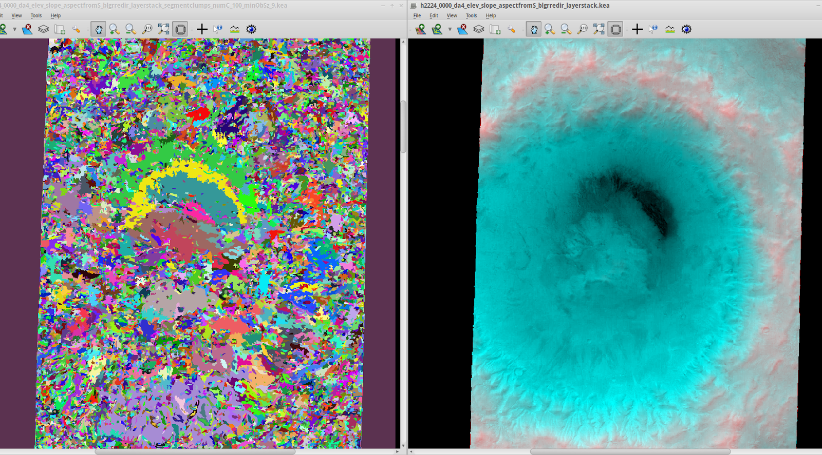RSGISLib segmentation does seem to group certain areas together such as the crater floor, and gullies, but I have quite a long way to go before having a method to identify the glacier-like features automatically.

Digital Terrain Model layerstack on Mars

I've begin to look at topographic analysis on Mars. Here's a HiRISE digital terrain model, with red coloured for higher elevations, green for steeper slopes, and blue for aspect.

This one is a Lineated Valley Fill in Deuteronilus Mensae.

Data from HiRISE website (NASA/JPL/University of Arizona/USGS) processed in GDAL and shown in Tuiview.

Edit - Importing into QGIS, showing the scale using a grid (units are in metres):
The elevation range is from -2681 to -1997 metres relative to Mars datum, and I've coloured slope in the range 0-30 degrees, and aspect 0-180 deg away from N.

Self-paced Introduction to QGIS and more on DEM segmentation

I have seen recently there is a self-paced course on QGIS from the  FOSS4Geo Academy . It is hosted on the open source Canvas Learning Network.

There are two modules so far, an introductory one, and a cartography one, with more coming soon.

Following on from my last post, here is the topography of the British Isles segmented using RSGISLib using a minimum object size of 65536 pixels.

This probably isn't a useful approach, since it took the computer about 9 hours to do this. I expect it is better to use smaller objects and aggregate them at the classification stage.

Here the mean segments are colourised using yellow for slope, and blue for elevation with a gaussian stretch as before.

 And here are the segments with a random colourisation.

Using a higher resolution (5m) DEM for mid-Wales, around the Aberystwyth, Dyfi estuary and Pumlumon area, aggregating to at least 1024 pixels (that is equivalent to a 160x160m square):

Object-based segmentation of topography with RSGISLib

The RSGISLib (Remote Sensing and GIS) Python library written by Pete Bunting and Daniel Clewley provides a number of features, among them segmentation of images to objects.

This can not only be applied to what one conventionally thinks of as images, but also topographic layers. I thought I'd practice this on Earth first before trying to do this for Mars as I will be for my dissertation.

Using Space Shuttle Radar data (freely available - I got it via the program Viking) I obtained the elevation of the British Isles (excluding Shetland) and using GDAL via QGIS and the command line, created slope and aspect layers. I then transformed the aspect to remove the discontinuity at 360-0 deg, using degrees from N, so that 180 is south facing, east and west are both 90 etc.

Using RSGISLib it is possible to segment to objects. Here I show some results of doing so, using a layerstacked image with elevation, slope and angle from N. I have set the minimum connected object size to 1000 pixels. With the topographic data gridded at 73m, this means objects about 5.5 sq. km or larger.


Visualisation is a gaussian stretch in TuiView, setting red to aspect, green to slope, and blue to elevation, showing mean values for each segment.

Now I show a few of the actual segments without the values, with colours assigned in RSGISLib for visualisation. It is possible to populate a Raster Attribute Table to add data to the segments for a land cover classification.

From the Isles of Scilly to the Isle of Wight:

Wales, and central England.

 Zooming in to mid Wales:

By changing the object size, it is possible to do this at different scales. This is part of the segmentation for a minimum object size of 16384 pixels (that is about 89 sq. km) equivalent to a square 9.5km a side:

The thing that makes geospatial data interesting is how what you see in it changes depending on what scale you look at it and how you visualise it.