An atlas of Wales in Welsh - data on OpenStreetMap

I recently saw a tweet by @mikeparkerwales about a new atlas of Wales in Welsh being prepared by @dafyddelfryn.

A Gaelic map of Scotland has also recently been produced by Paul Kavanagh.
As well as my own work, there is also Justin Cozart's map of Cornwall in Cornish.

I have produced a set of cycling maps of Wales where I used the placenames from OpenStreetMap. My procedure was to prefer the Welsh name, i.e. use the name:cy tag where it existed, otherwise the name tag.

I couldn't actually remember how I had got the Welsh names, since they are not on the standard shapefile downloads from geofabrik.de that I usually have used.

However the full set of tags are available by using the .pbf file available at download.geofabrik.de/europe/great-britain.html which needs a little more work, firstly to convert to the full XML by osmconvert, and then to turn that into SpatialiteDB format. The tutorial here explains a little of how this is done.
This process can be horribly inefficient, since a large .pbf file is downloaded, which is processed into an even larger XML. I think there are other ways to do it which avoid this which I may look into in future.

For the Welsh names, it is necessary to look for the name and name:cy tags, and maybe also name:en tags, which exist for some places, though this is usually just a duplication of name. A very few places have an alt_name:cy tag, where there is more than one Welsh name current for a particular place.





See also WikiProject Wales on the OpenStreetMap wiki. Unfortunately neither the Welsh language OpenStreetMap rendering at http://brasskipper.org.uk/cyosm or the multilingual test page by Jochen Topf currently seem to be working.

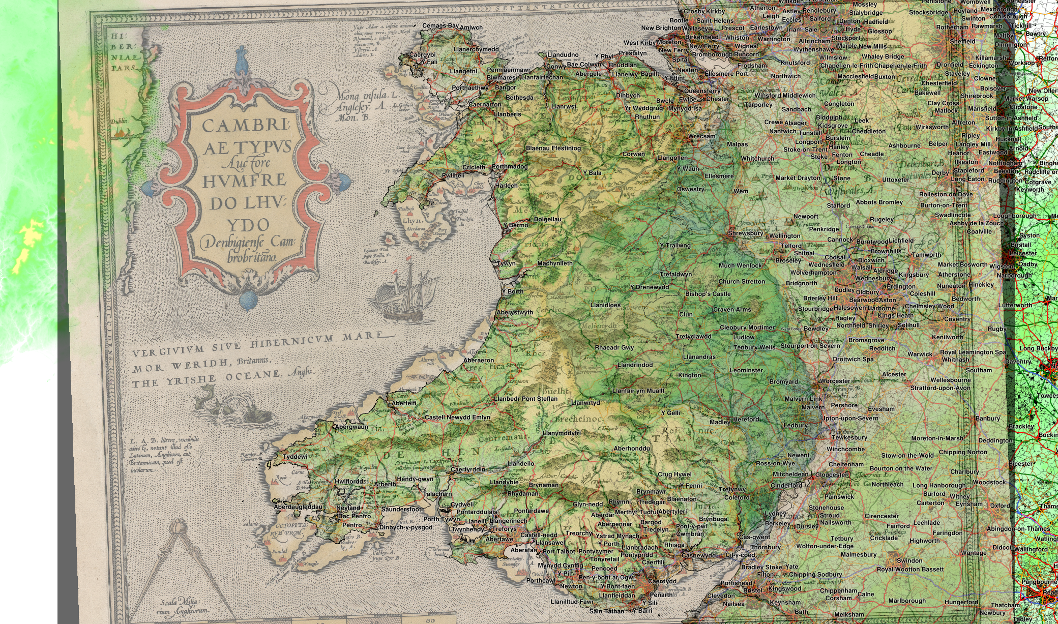
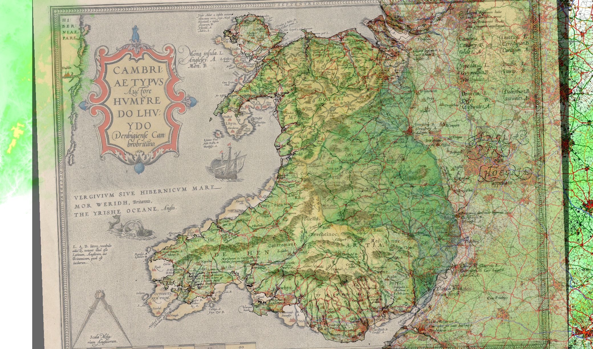
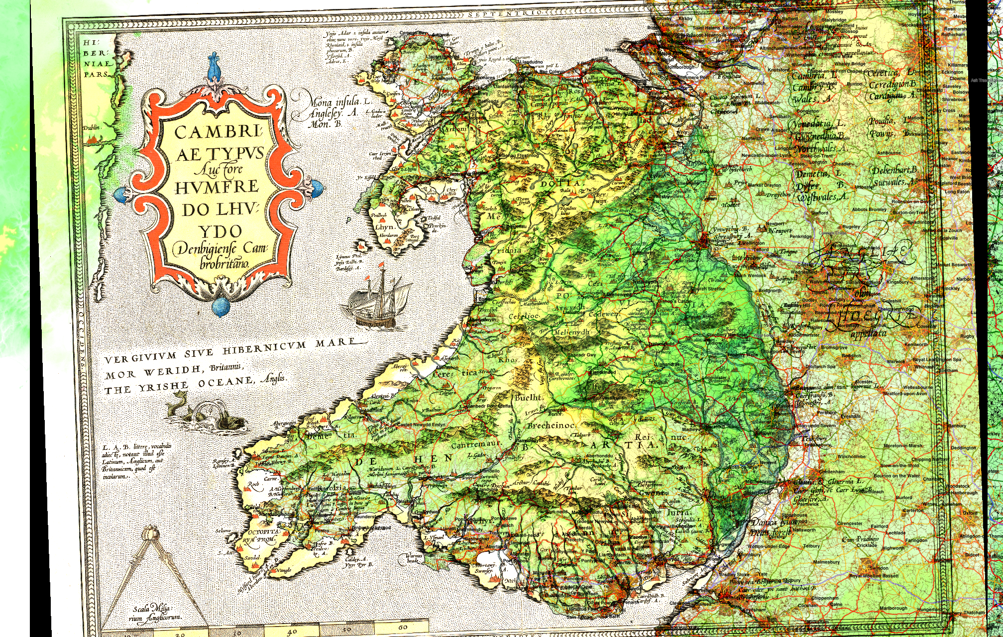
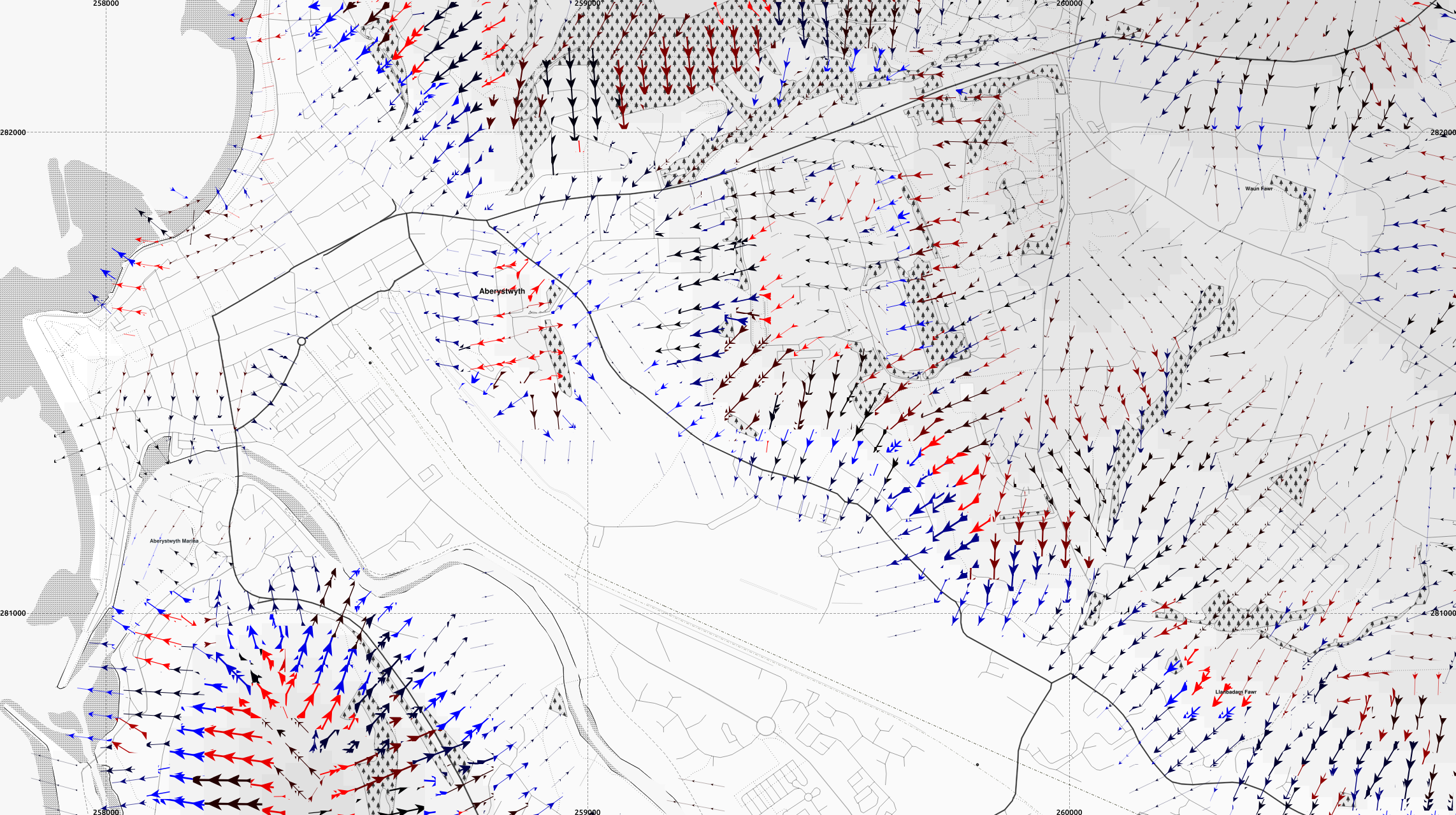
Here are some basic renderings of placenames in QGIS, using the places.shp from the geofabrik.de shapefile of Wales, and 'joining' this to the name:cy, name:en and alt_name:cy tags from the Spatialite version.

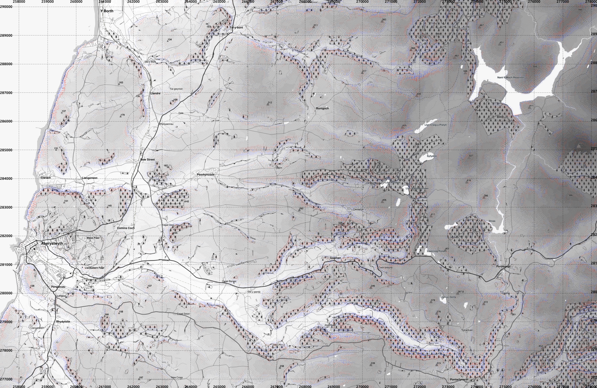
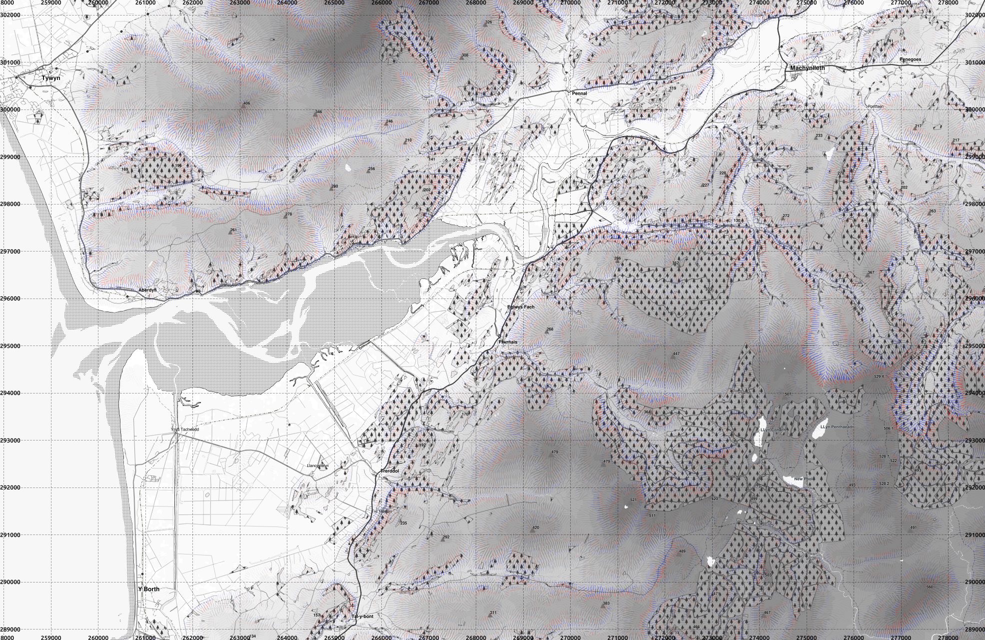
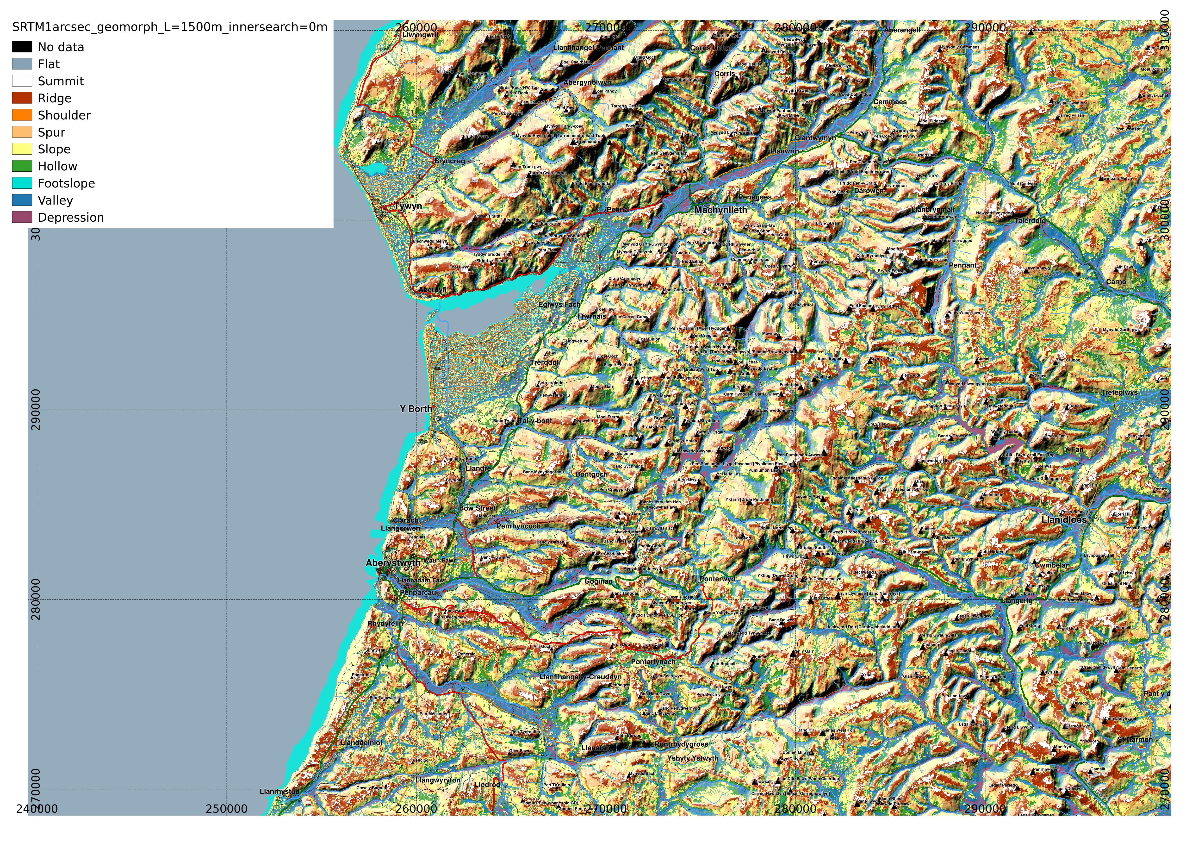
Mid-Wales. Most names only have the name tag, and where a separate name:cy tag exists, the name tag is generally the English name, although in the case of Ffwrnais, it is a bilingual form. Where name:en exists, it is usually a duplicate of name, but in one case (Pontfaen /  Forge), name:cy and name:en tags but no name. Barmouth has an alt_name:cy tag of "Y Bermo" defined.

Holyhead. Similarly where name:cy exists, name is sometimes the English version and sometimes a bilingual form.

Cardiff. Many bilingual names are in evidence, the general practice here seems to be to use name:cy for the Welsh name and name for the English name, and where name:en exists, it is usually simply a duplicate of name.

Bridgend. The remaining two places in the populated places shapefile that have an alt_name:cy defined are here.

False colour composite of Sentinel 2 - 30.05.16

After using the script in the previous post to create a layerstacked .kea file for each "granule" within the Sentinel 2 images I downloaded, I created a false colour composite mapping band 11 (SWIR 1610nm) to red, band 8 (NIR, broadband centred around 842nm) to green, and band 4 (red 665nm) to blue.

See https://sentinel.esa.int/web/sentinel/user-guides/sentinel-2-msi/resolutions/spatial for a description of the bands available in Sentinel 2.

Here is a mosaic made in Tuiview:

After some issues with opening .kea files in QGIS (due to having reinstalled Ubuntu recently and needing to recompile KEAlib and then finding that due to being compiled against GDAL 2.1 libraries it didn't work in QGIS which was using GDAL 1.11),  I sorted this out, and have a QGIS project file showing the image. I also show some placenames from OpenStreetMap, and hill names from www.hill-bagging.co.uk for context.

Some screenshots of QGIS are shown below:

Aberystwyth area

Bodmin Moor, Cornwall. Road construction can be seen at the lower left.

Falmouth and surrounding area.

Snowdon

Truro area.

Plymouth, Saltash and Torpoint and the Rame peninsula

A clear day for Sentinel 2 satellite image of Cornwall

The ESA Copernicus programme includes the twin satellites Sentinel 2A and Sentinel 2B which have a multiband sensor. Details can be found here: https://sentinel.esa.int/web/sentinel/missions/sentinel-2.

Sentinel 2A has already been launched and is taking data, and Sentinel 2B will be launched later in 2016.

The Scientific Data Hub provides access to the data, although there is also access via an API, and via Amazon Web Services, and USGS Earth Explorer (currently some time behind).

Until recently, the images of Cornwall had been mostly heavily affected by cloud, although there was a better one taken on 30th May 2016.

A composite of bands 2, 3, and 4 (not atmospherically corrected) showing west Cornwall.

A composite of bands 2, 3 and 4 (not atmospherically corrected) around Aberystwyth in mid-Wales.

A Python script, using RSGISlib to stack Sentinel2 images into a band-stacked .kea file:

# David Trethewey 01-06-2016
#
# Sentinel2 Bands Stacker
# Uses visible, NIR, SWIR bands
# 
# Assumptions:
#
# the .jp2 files are in the current directory
# that this script is being run from
#
# there is only one Sentinel2 scene in the directory
# and no other jp2 files
#  
# Converts jp2 files of each band to single stacked file
#  
# imports
import rsgislib
import rsgislib.imageutils
import os.path
import sys

# image list
# find all *.jp2 files in the current directory
directory = os.getcwd()
dirFileList = os.listdir(directory)
# print dirFileList

jp2FileList = [f for f in dirFileList if (f[-4:].lower()=='.jp2')]

bands = ['01', '02', '03', '04', '05', '06', '07', '08', '09', '10', '11', '12', '8A']
# bands that are already at 10m resolution
bands_10m = ['02', '03', '04', '08']

# resample other bands to resolution of blue image (B02)
bands_toberesam = [b for b in bands if b not in bands_10m]

# identify the band number by counting backwards from the end in the filename
Bands_VIS_NIR_SWIR_FileList = [f for f in jp2FileList if (f[-6:-4] in bands)and(f[-7]=='B')]

# list of bands to be resampled
Bands_resam_FileList = [f for f in jp2FileList if (f[-6:-4] in bands_toberesam)and(f[-7]=='B')]

# find the filename of the blue image
blue_image = [f for f in jp2FileList if (f[-6:-4] == '02')and(f[-7]=='B')][0]

# bands to be resampled 20m --> 10m
# 05, 06, 07, 8b, 11, 12
# bands to be resampled 60m --> 10m
# 01, 09, 10

for b in Bands_resam_FileList:
    print("resampling band {q} to 10m".format(q=b[-6:-4]))
    outFile = b[:-4]+'_10m.kea'
    rsgislib.imageutils.resampleImage2Match(blue_image, b, outFile, 'KEA', 'cubic')
    Bands_VIS_NIR_SWIR_FileList.remove(b)
    Bands_VIS_NIR_SWIR_FileList.append(outFile)

Bands_VIS_NIR_SWIR_FileList = sorted(Bands_VIS_NIR_SWIR_FileList)

fileNameBase = blue_image[:-7]

# Sentinel2 bands
bandNamesList = ["B1Coastal443nm", "B2Blue490nm", "B3Green560nm", "B4Red665nm", "B5NIR705nm", "B6NIR740nm",
                 "B7NIR783nm", "B8NIR_broad842nm", "B9NIR940nm", "B10_1375nm", "B11_SWIR1610nm",
                 "B12_SWIR2190nm", "B8A_NIR865nm"]

#output file name
outputImage = fileNameBase + 'B'+''.join(bands)+'_stack.kea'

#output format (GDAL code)
outFormat = 'KEA'
outType = rsgislib.TYPE_32UINT

# stack bands using rsgislib 
rsgislib.imageutils.stackImageBands(Bands_VIS_NIR_SWIR_FileList, bandNamesList, outputImage, None, 0, outFormat, outType)
# stats and pyramids
rsgislib.imageutils.popImageStats(outputImage,True,0.,True)

# remove individual resampled 10m files
print("removing intermediate resampled files")
for b in Bands_resam_FileList:
    outFile = b[:-4]+'_10m.kea'
    os.remove(outFile)

Slope lines from segmented digital elevation model - after upgrade to QGIS 2.12.1

I mentioned previously that I used QGIS to draw lines in the direction of slope, where I had a segmented layerstack which included elevation, slope, aspect and 2 curvature layers (longitudinal and cross-sectional). This was done with RSGISlib in a similar way to my Mars work.

There was an bug with QGIS 2.12 that meant the plotting of arrows didn't work but with QGIS 2.12.1 this seems to be working again. It still takes a long time to render with the SVG marker, even with 32GB RAM and a quad-core system.

Here are a few examples:

Truro area in Cornwall. The slopes are marked with arrowed lines, with steeper slopes marked more thickly, and red for convex, and blue for concave slopes.

A closer zoom into the city.

Around Falmouth, including Pendennis Head

Falmouth again, with grayscale elevation.

Aberystwyth, Ceredigion, Wales:

I show here several QGIS screenshots, at 1:10000 or larger scale, since the rendering of the arrows becomes very slow beyond 1:10000.

Ynys Las and part of Borth Bog (Cors Fochno). This is mainly a flat area so most segments do not have lines shown.

Borth itself, a little to the south

Clarach Bay, and Wallog, and Bow Street

Aberystwyth town and main university campus are here shown, along with Pendinas hillfort, Penparcau, and Llanbadarn Fawr.

Cadair Idris - a textbook glacial landscape

Showing the arrows downslope only.

Adding in the slope parallell lines but making the arrowheads smaller.

At 1:20000 this takes a long time to render on the map canvas in QGIS.

A version with only the lines renders much faster.

Using contours instead of shading to indicate elevation.

Georeferencing a map from 1574

I saw the National Library of Wales had digitised a map of Wales produced circa 1574 by Humphrey Llwyd, and uploaded a copy to Wikimedia commons.

I decided to try georeferencing it to a modern map based on OpenStreetMap data using the QGIS georeferencer:

Overlaying 1574 map with transparency shows the variability in the accuracy of the map. full-size version

Removed modern town names to show 1574 map more clearly. full-size version

I chose a variety of places around Wales and the border areas shown on the map, including Cardiff, Newport, St. Davids, Aberystwyth, Holyhead, Liverpool, Shrewsbury, Hereford.

The result looks more accurate than I expected, with Aberystwyth and Shrewsbury being almost exactly referenced, and several other places with small errors.

According to the author Graham Robb, Whitchurch in Shropshire was the prime longitude meridian for the British Druids in the Iron Age, and is named as "Mediolanum" by Ptolemy in the 2nd century. Aberystwyth (or more exactly, the Pendinas hillfort) was also an important location within their navigation system apparently, being both on a longitude meridian and latitude paralell.

Update: QGIS layer blending

Changing the layer blending method to a "Hard light" overlay rather than semi-transparency makes for a slightly clearer result I think:

full-size version

Maps of Wales with slope arrows

Here are a couple of maps of Aberystwyth, and Cadair Idris, with the RSGISlib segmented digital elevation model.
Slope direction is shown by arrows, and coloured in the same scheme as previously with thicker arrows for steeper slopes, and longitudinal curvature indicated with convex slopes red and concave blue.

1:10000 seems about the limit of the smallest scale that QGIS will cope with the arrowed lines. Beyond that the computer just hangs - slope lines without arrows can be plotted without problem.

Aberystwyth town centre, and the university campus. full-res version

Cadair Idris. This is a textbook example of a glacial landscape in the British Isles. full-res version

Aberystwyth area and Rheidol Valley. full-res version

Dyfi Estuary showing Borth, Tywyn and Machynlleth. full-res version

To readers: are there any requests of areas you would like to see?

The processed data currently includes the following area though I also have the whole of British Isles (except most of Shetland) DEM from 1 arcsec SRTM (and could download anywhere up to 60° latitude) but not processed to create slope curvature layers and segmented.

Pen-y-fan area, Brecon Beacons

Pen-y-fan main summit to the right of centre, showing the slopes convex at the top, but generally concave further down. full-res version

Broader context at 1:40000. full-res version

A map of Aberystwyth using lines along slope direction to indicate slope

This is another map like the ones in yesterday's post, this time of the town of Aberystwyth in Wales, and a little of the area surrounding it.

I have altered the spacing of the slope lines, which are now 20m apart, with grid squares shown at 1km size.

Roads as usual come from OpenStreetMap, with OS Vector Map foreshore, woodland, plus tidal and inland water (the labels of these are from OpenStreetMap - possibly a dangerous thing to do, if something is in OSM but not OS VectorMap there will be a labelled object that is not mapped!).

Hill peaks are from www.hill-bagging.co.uk, plotting all greater than 150m with more than 20m drop.

As before, the steepness of hills is indicated by the width of the slope lines, in this version, they are plotted with 10*((Slope_deg_Mean - 2.25) / 45.0) metres width, if the slope exceeds 2.25 degrees, and if not omitted.

That is no lines are plotted where the average slope of the segment is less than 1 in 20, and increase in width up to 19.5m as slope approaches 90 degrees. So a vertical cliff will be almost solid red.

They are plotted in the direction of the mean aspect of the segment. This is the real aspect, not the absolute distance from north.
It is possible that a segment facing north may for example have half of it at 1 degree east, and the other half at 359 degrees. Thus the average would be at 180 degrees. This doesn't matter because the lines have no arrows on them.
However if you have 3/4 of it facing 359 degrees, and 1/4 facing 1 degree, then it would produce spurious results, therefore slope direction may be dubious on north-facing slopes.

Aberystwyth, with the Ystwyth and Rheidol rivers, and Clarach Bay at the top. There are certain areas where a north-facing slope is given a spurious east-west slope line, such as the north-facing slope at the top of this image at Clarach.

When I originally did this, I thought that the excess division of segments along the N/S line when I segmented using the original aspect, rather than the absolute angle from north, was a problem. However for this purpose, dividing segments that cross the 360/0 degree discontinuity helps some of the north-facing slopes avoid spurious east-west 'mean aspect' of segments:

Compare the north-facing slopes to the previous image.

The segment boundaries plotted for illustrative purposes.

A bit more on geomorphons, varying the 'inner search radius'

I had originally posted maps of DEMs of Cornwall and the Aberystwyth area of mid-Wales processed using Tomasz Stepinski et al.'s geomorphon method as descibed in the papers of: Stepinski+Jasiewicz 2011, Jasiewicz + Stepinski 2013.

Since then I have become aware of the 1 arcsecond SRTM data being available, so I have recalculated the geomorphons and here show the map of the same area of mid-Wales that the landcover assignment from my MSc was concerned with.

Using the search distance L=1500m, as did T. Stepinski in his geomorphon map of Poland (user guide), I varied the 'inner search radius' which determines the minimum distance the software looks, using 0, 2 and 4 cells. 1 cell is ~ 24m in the SRTM 1 arcsec data after conversion to OS grid reference coordinates.

Inner search radius 0m

In some of the flatter areas results are difficult to interpret. full-resolution image.

Inner search radius 2 cells (~50m)

Looking in Borth Bog, more of the area is shown as 'Flat' full-resolution image.

Inner search radius 4 cells (~100m)

As the inner search radius is expanded to 4 cells, most of the possibly spurious peaks in the flat area of Borth Bog disappear. full-resolution image.

I expect it would be interesting to combine it with the segmentation and classification with RSGISlib and to examine correlations between the landscape position of a location, and the land-cover.

A little more on the "omission error" for the woodland areas

To have a bit more of a look at the areas that are woodland in OS VectorMap and not classed as woodland in the classification, I here show where these areas are on the satellite images, and the classes that these areas are in fact assigned.

June 2006

Showing the areas indicated as woodland in OS VectorMap but not by the classification outlined in black, overlaid on the Landsat 7 image from 9th June 2006 (bands 5,4,3). large version

Showing the actual classifications the "omission error" areas were assigned. large version

March 2007

Showing the areas indicated as woodland in OS VectorMap but not by the classification outlined in black, overlaid on the Landsat 7 image from 24th March 2007 (bands 5,4,3). large version

Showing the actual classifications the "omission error" areas were assigned. larger version

September 2013

Showing the areas indicated as woodland in OS VectorMap but not by the classification outlined in black, overlaid on the Landsat 8 image from 24th September 2013 (bands 6,5,4). Some areas that display in pink here appear to be recently felled forest areas that have a weak reflectance in NIR (shown in green), but strong in SWIR1 (shown in red) with some reflectance in red (shown in the blue channel here). large version

Showing the actual classifications the "omission error" areas were assigned, and the 'cloud' areas. Some shaded areas are spuriously being classified as water. large version

Errors in the land cover assessment

Last time, I mentioned I was going to compare the ground control points to the classification.
Before I do that, I thought I'd compare the extents of classified woodland and water to OS VectorMap data.

I show the "commission error" - where the classification indicated something where OS VectorMap didn't, and "omission error" where OS VectorMap indicated something but the classification didn't.
Not all of the difference may be error in the classification, there may have been real change on the ground between the epoch of the image and the OS VectorMap data, or what is marked out as a woodland areas on VectorMap may include clearings, felled areas, or partially forested areas that were often classified as "Mosaic".

June 2006

RGB (9th June 2006)

NIR:SWIR1:Red 9th June 2006

 

large version There are a few areas of cloud shadow and other areas falsely classified as water. In addition there are some areas of cloud which may not be real. The woodland is generally underpredicted relative to OS VectorMap, the "omission error" areas are often classified as "Mosaic".

March 2007

 

RGB 24th March 2007

NIR:SWIR1:Red 24th March 2007

large version This is perhaps the most accurate of the woodland classifications, though some of the woodland areas are missed particularly in the east of the image (where perhaps cloud is interfering to some extent) and is often classified as "mosaic". There are a few areas of bogusly classified water in topographic shadow areas

 

September 2013

RGB (24th September 2013)

NIR:SWIR1:Red

large version Extensive areas of thin cloud appear in this image, woodland is overpredicted relative to OSVectorMap. It is likely that, late in the growing season, other vegetation has increased in NDVI and is perhaps masquerading as forest, or the subtle shadows of thin cloud are affecting the classification. Again some topographic shadowed areas are erroneously classed as water.

It is evident that the kind of first-order adjustment for seasonal change in NDVI etc. is not really adequate to prevent large shifts between classes, instead it is likely to be necessary to examine each landcover class in detail to see how its spectral properties change across the growing season.