Showing posts with label RSGISLib. Show all posts

Sunday, 4 June 2017

Computer troubles and further updates to TaklowKernewek tools

My desktop computer is currently incapacitated, it has for the past day and a half been resizing a NTFS partition after I made the decision, after breaking my QGIS installation while attempting to upgrade it to 2.18, to go back to a dual-boot system rather than a Windows virtual machine running in Ubuntu. Meanwhile I had also broken my netbook because it crashed while trying to upgrade to Ubuntu 17.04. I fixed this by doing a reinstall from a bootable USB stick using the UbuntuMATE iso, formatting only the root partition leaving data in /home intact.

This shouldn't deter anyone from using QGIS, or Ubuntu, just that I was doing odd things with GDAL and kealib, making myself able to use multiband .kea files  in QGIS running with the system environment variables, but use conda to run RSGISLib in Python 3, and also conda to run the European Space Agency's SNAP toolbox to process Sentinel 2 images.
There was a resulting mismatch between different versions of GDAL which caused problems when I tried to update to QGIS 2.18, which failed due to conflicting dependencies, and then trying to revert to 2.14 also failed, so therefore QGIS no longer worked at all.
With my netbook, I had installed so much on it that the root partition was close to full and I think that was what started causing problems.

Fortunately all data is backed up on external drives.

However it is not so easy to do much mapping work on my netbook, although I do now have QGIS 2.18 installed on it, but I have done a bit more on TaklowKernewek, including making the netbook mode work for more of the apps, and developing the mathematics quiz app.

The netbook modes were modified to allow the corpus statistics app, and a couple of others to fit the screen of my netbook (EeePC 1005HA), by adjusting font sizes as well as some input/output box heights.
Inflecting the verb 'covhe' (in SWF Tradycyonal) - Cornish for 'remember'


Inflecting the verb 'covhe' (in SWF Tradycyonal) - Cornish for 'remember'


Basic translation memory using Skeul an Yeth 1 example sentences. The font size of three of the four buttons has been shrunk a little so that labels do not grow bigger than the box itself.

more of the output

some further output of the translation memory


word frequency table for words of 5 or more letters in 'Origo Mundi'. The font sizes are quite small to read to make sure that the boxes do not fall off the bottom of the screen.
The word frequency bar chart has been tweaked as to not use white as a colour, since matplotlib may not always outline the bars.

counting syllables


Transliterating from Kernewek Kemmyn to Standard Written Form. It is possible that goelann should instead go to goolan in SWF, it certainly did in 2008 SWF, and may still do so despite being a multisyllable word.

Mathematics Quiz app

A new difficulty level allow input numbers up to 100, and the GUI has been adjusted to work better on smaller screens (though further work on this may be needed).
The options radio buttons have been consolidated into one column in the GUI

The program now reports back the answer to the previous question that you gave if you were correct as well as if you were wrong. This still looks a little confusing since the question now in the upper box is the second question whereas the answer is for the first. If you get a question right, you get 1 point. The bonus for speed has been reduced compared to earlier versions, to get any speed bonus at all you need to answer within 10 seconds.

'Pur gales' allows the computer to choose numbers up to 100, in this version the addition and subtraction are shown as symbols, due to possible confusion with 'ha' internal to the number such as 'dew ha dew ugens' (42). 'tri ha dew ugens marnas dew ha dew ugens' might be interpreted as 43 - 2 + 40 = 81 rather than 43 - 42 = 1.

There is a need to make some further adjustments to the Tkinter GUI code since at present the widgets aren't filling the window after it is maximized.

Sunday, 2 October 2016

Souness Martian Glacier Top Trumps

I have made some additions and improvements to my website that lists the glacier like forms on Mars detailed by Colin Souness, and presents Mars Express data and links to HiRISE coverage from the Mars Reconnaisance Orbiter.

See an example here:
taklowkernewek.neocities.org/mars/sounesstoptrumps_js.html?S1003

The data is processed using some obsfucated Python code, which uses a combination of RSGISlib, GDAL via the command line and ImageMagick to provide a subset of the HRSC data to a bounding box of the 'context' shapefile of each Souness glacier (relying on the manual identification of the 'best' HRSC footprint with DTM coverage in the dissertation work).

This presents the panchoromatic nadir image, digital terrain model, a layerstack combining HRSC image and DTM, overlaying the classifier as calculated for glacier head areas in my dissertation, or else falling back to the Mars Global Surveyor coverage in which case a lower resolution image and DTM only are available.

Overlap with HiRISE, and HiRISE anaglyphs/DTM with the extents and wider 'context9' shapefiles were automatically identified, and also the level 3 HRSC images (the ND3 links).

If you open two browser windows, you and a friend can actually play the game of Top Trumps by the first player drawing a 'card' with the choose random button, choosing a category to play, and then the second player presses their random button and see if they beat them.

It is up to you if you want to play with north good, or high elevation good etc.

The page showing one of the Souness glacier-like forms in the southern hemisphere on Mars.

Showing the High Resolution Stereo Camera aboard Mars Express digital terrain model.

Indicating HiRISE coverage with a yellow overlay, which shows that there isn't coverage over the footprint of this object, but there is in the general vicinity. See below for an example of another Souness object where there is both HiRISE and anaglyph coverage.

A layerstack consisting of the panchromatic nadir image from HRSC (mapped to red), the slope of the DTM (green), and the elevation (blue). These are locally scaled within the bounding box of the 'context' shapefile, which is the white box visible (the extent) scaled up by a factor of three.

The data table. Links are given to Mars Express data from the Nasa Mars Orbital Data Explorer, Arizona State University, and Freie Universität Berlin, MRO context camera also from Arizona State University and HiRISE data from University of Arizona.
Elevation profile using the h2279 HRSC terrain model.

Slope profile using the h2279 HRSC terrain model.
Object number 716 in the Souness catalog has overlay with HiRISE and HiRISE anaglyph footprints, which are distinguished by being written in bold in the table.

Friday, 5 August 2016

Using QOSM to provide OpenStreetMap basemap in QGIS for my slopelines project

In previous posts I have described how I have used a segmented DEM with RSGISlib, a method originally developed as part of my MSc dissertation on Martian glaciers, for visualising slopes on Earth.

I have been looking at these again, and have produced a few maps with the QOSM plugin, which dynamically loads OpenStreetMap tiles into QGIS.

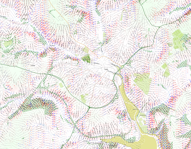
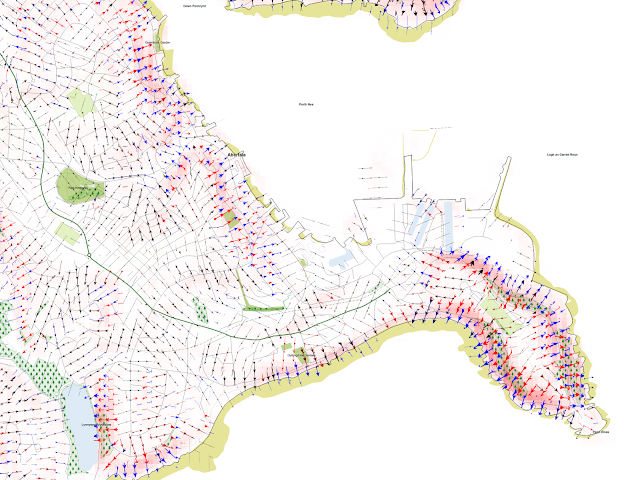
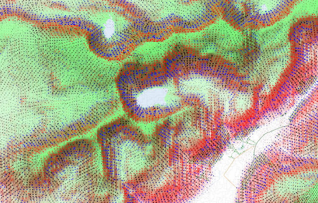
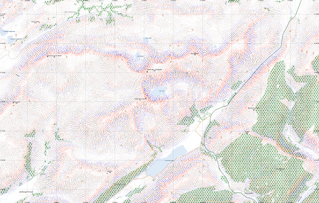
These maps below were produced with the Thunderforest Outdoors rendering. The slopelines are as previously, red for convex slopes, blue for concave, with thicker lines denoting steeper slopes.

Previous versions of this had used a version of OpenStreetMap that I was preparing myself from the source data within QGIS. Using the basemap tiles I can focus on adapting the visualisation of the slope lines themselves a bit more.

Bodmin Moor

Camborne and Redruth, including Carn Brea and Portreath

Penzance

Truro

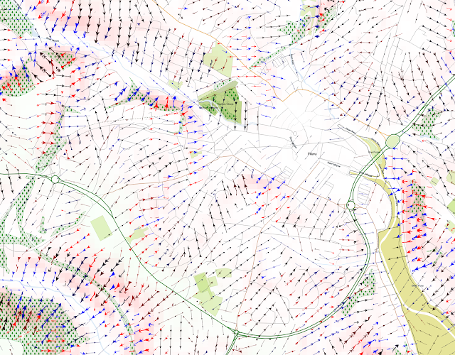
A close up of Truro
For a while I thought the QGIS bug I found had recurred which meant that the arrows had disappeared. However it was something wrong in my data dependent styling, not sure how it happened. Once fixed, I show the slope direction with arrows, which is only possible up to about 1:10,000 otherwise the rendering struggles:

Indicating the downslope direction with arrows.

Delabole, showing the slate quarry.
St. Ives

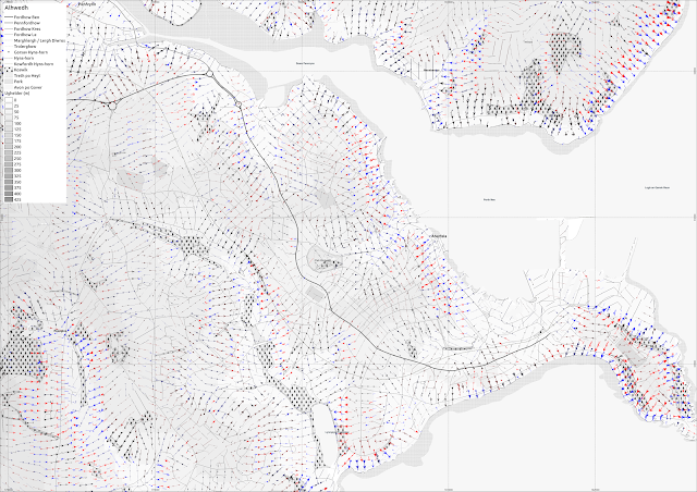
Aberystwyth, Wales

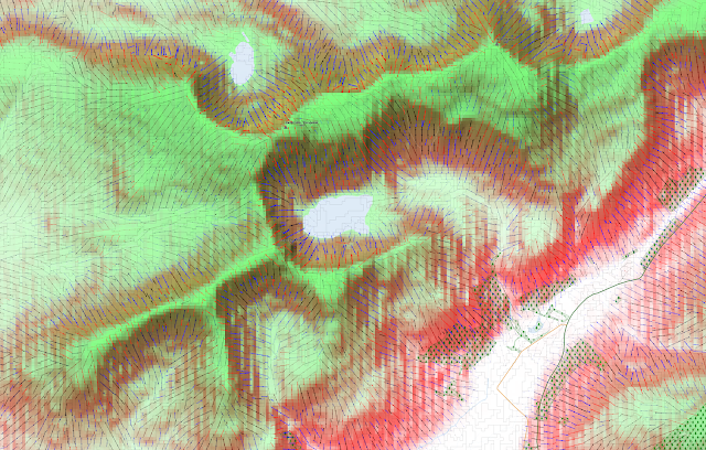
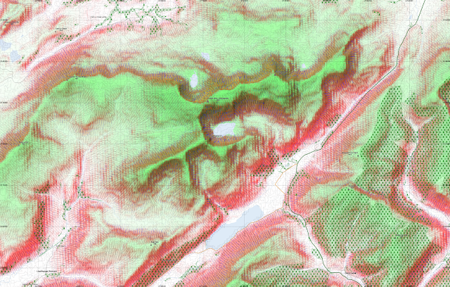
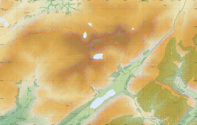
Cadair Idris, Wales

A wider view of Cadair Idris, too small a scale to allow plotting the arrows.


Pen y Fan, Brecon Beacons, Wales


Monday, 6 June 2016

Atmospheric correction of Sentinel 2 images

I recently downloaded the Sentinel Application Platform including the Sentinel 2 Toolbox.

This looks to be a fairly fully featured image processing program, but what I was most interested in doing is the atmospheric correction for the Sentinel2 images I recently downloaded.

The Sentinel 2 'sen2cor' plugin accomplishes this, which wasn't too difficult to install, making use of anaconda to manage the various dependencies. Once I managed to get the environment variables set, and have it find all of the libraries it pretty much just worked.

After this, I tried using my own script for stacking the bands, which came out with a non-georeferenced image. I then noticed I could save the layerstacked image as a GeoTIFF/BigTIFF from within SNAP. A single 'granule' of Sentinel2 resampled to 10m produced a 9GB GeoTIFF, so I converted to KEA with gdal_translate.

Sentinel 2 image processed to Level2A, with SNAP and sen2cor. Bands B11/B8/B4
Zooming in on the Truro area. Penryn can be seen at the lower-left.

Using my rsgislib-landexplorer program to juxtapose geotagged ground-level images with Sentinel2
The same as above, but the non-atmosphere corrected version of the Sentinel2 image.

Wednesday, 1 June 2016

A clear day for Sentinel 2 satellite image of Cornwall

The ESA Copernicus programme includes the twin satellites Sentinel 2A and Sentinel 2B which have a multiband sensor. Details can be found here: https://sentinel.esa.int/web/sentinel/missions/sentinel-2.

Sentinel 2A has already been launched and is taking data, and Sentinel 2B will be launched later in 2016.

The Scientific Data Hub provides access to the data, although there is also access via an API, and via Amazon Web Services, and USGS Earth Explorer (currently some time behind).

Until recently, the images of Cornwall had been mostly heavily affected by cloud, although there was a better one taken on 30th May 2016.

A composite of bands 2, 3, and 4 (not atmospherically corrected) showing west Cornwall.

A composite of bands 2, 3 and 4 (not atmospherically corrected) around Aberystwyth in mid-Wales.
A Python script, using RSGISlib to stack Sentinel2 images into a band-stacked .kea file:

# David Trethewey 01-06-2016
#
# Sentinel2 Bands Stacker
# Uses visible, NIR, SWIR bands
# 
# Assumptions:
#
# the .jp2 files are in the current directory
# that this script is being run from
#
# there is only one Sentinel2 scene in the directory
# and no other jp2 files
#  
# Converts jp2 files of each band to single stacked file
#  
# imports
import rsgislib
import rsgislib.imageutils
import os.path
import sys

# image list
# find all *.jp2 files in the current directory
directory = os.getcwd()
dirFileList = os.listdir(directory)
# print dirFileList

jp2FileList = [f for f in dirFileList if (f[-4:].lower()=='.jp2')]

bands = ['01', '02', '03', '04', '05', '06', '07', '08', '09', '10', '11', '12', '8A']
# bands that are already at 10m resolution
bands_10m = ['02', '03', '04', '08']

# resample other bands to resolution of blue image (B02)
bands_toberesam = [b for b in bands if b not in bands_10m]

# identify the band number by counting backwards from the end in the filename
Bands_VIS_NIR_SWIR_FileList = [f for f in jp2FileList if (f[-6:-4] in bands)and(f[-7]=='B')]

# list of bands to be resampled
Bands_resam_FileList = [f for f in jp2FileList if (f[-6:-4] in bands_toberesam)and(f[-7]=='B')]

# find the filename of the blue image
blue_image = [f for f in jp2FileList if (f[-6:-4] == '02')and(f[-7]=='B')][0]

# bands to be resampled 20m --> 10m
# 05, 06, 07, 8b, 11, 12
# bands to be resampled 60m --> 10m
# 01, 09, 10

for b in Bands_resam_FileList:
    print("resampling band {q} to 10m".format(q=b[-6:-4]))
    outFile = b[:-4]+'_10m.kea'
    rsgislib.imageutils.resampleImage2Match(blue_image, b, outFile, 'KEA', 'cubic')
    Bands_VIS_NIR_SWIR_FileList.remove(b)
    Bands_VIS_NIR_SWIR_FileList.append(outFile)

Bands_VIS_NIR_SWIR_FileList = sorted(Bands_VIS_NIR_SWIR_FileList)

fileNameBase = blue_image[:-7]

# Sentinel2 bands
bandNamesList = ["B1Coastal443nm", "B2Blue490nm", "B3Green560nm", "B4Red665nm", "B5NIR705nm", "B6NIR740nm",
                 "B7NIR783nm", "B8NIR_broad842nm", "B9NIR940nm", "B10_1375nm", "B11_SWIR1610nm",
                 "B12_SWIR2190nm", "B8A_NIR865nm"]

#output file name
outputImage = fileNameBase + 'B'+''.join(bands)+'_stack.kea'

#output format (GDAL code)
outFormat = 'KEA'
outType = rsgislib.TYPE_32UINT

# stack bands using rsgislib 
rsgislib.imageutils.stackImageBands(Bands_VIS_NIR_SWIR_FileList, bandNamesList, outputImage, None, 0, outFormat, outType)
# stats and pyramids
rsgislib.imageutils.popImageStats(outputImage,True,0.,True)

# remove individual resampled 10m files
print("removing intermediate resampled files")
for b in Bands_resam_FileList:
    outFile = b[:-4]+'_10m.kea'
    os.remove(outFile)


Saturday, 19 December 2015

Slope lines from segmented digital elevation model - after upgrade to QGIS 2.12.1

I mentioned previously that I used QGIS to draw lines in the direction of slope, where I had a segmented layerstack which included elevation, slope, aspect and 2 curvature layers (longitudinal and cross-sectional). This was done with RSGISlib in a similar way to my Mars work.

There was an bug with QGIS 2.12 that meant the plotting of arrows didn't work but with QGIS 2.12.1 this seems to be working again. It still takes a long time to render with the SVG marker, even with 32GB RAM and a quad-core system.

Here are a few examples:

Truro area in Cornwall. The slopes are marked with arrowed lines, with steeper slopes marked more thickly, and red for convex, and blue for concave slopes.

A closer zoom into the city.
Around Falmouth, including Pendennis Head
Falmouth again, with grayscale elevation.

Aberystwyth, Ceredigion, Wales:

I show here several QGIS screenshots, at 1:10000 or larger scale, since the rendering of the arrows becomes very slow beyond 1:10000.


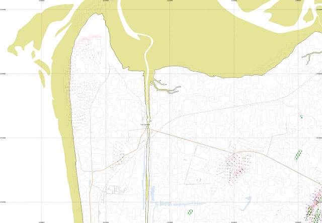
Ynys Las and part of Borth Bog (Cors Fochno). This is mainly a flat area so most segments do not have lines shown.
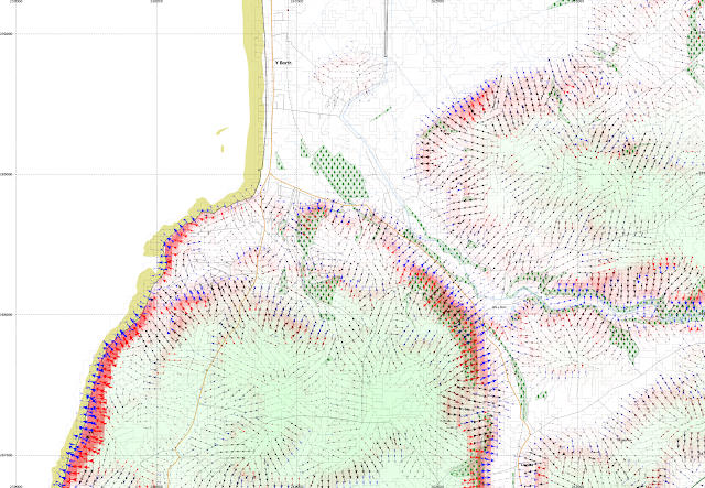
Borth itself, a little to the south
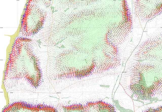
Clarach Bay, and Wallog, and Bow Street

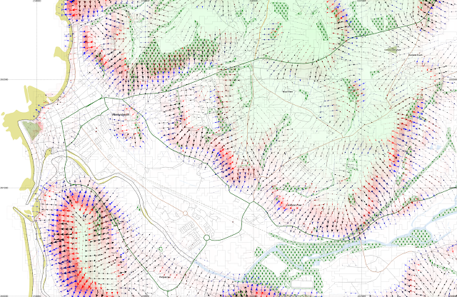
Aberystwyth town and main university campus are here shown, along with Pendinas hillfort, Penparcau, and Llanbadarn Fawr.

Cadair Idris - a textbook glacial landscape

Showing the arrows downslope only.

Adding in the slope parallell lines but making the arrowheads smaller.

At 1:20000 this takes a long time to render on the map canvas in QGIS.
A version with only the lines renders much faster.

Using contours instead of shading to indicate elevation.