Indicating curvature layers on the slope lines map

In the segmentation discussed in the previous two posts, as well as mean elevation, slope and aspect, I also have two curvature layers, longitudinal, and cross-sectional curvature that I calculated in LandSerf. The definitions of these are explained in the PhD thesis of Jo Wood, the author of LandSerf.

I thought to indicate longitudinal curvature using colour, shading convex slopes in red and concave in blue. Cross-sectional curvature is indicated with dots, which are white for diverging slopes and black for converging. Both of these are normalised by the square root of the segment area relative to the minimum segment area.

Newquay in Cornwall. Convex slopes appear in red, concave in blue.

Cadair Idris. Some strongly curved areas create very large dots that fill entire segments above Llyn Cau

Rescaling the dots to half their radius.

Normalising the radius of the dots by the slope. i.e. reduce dots on steep slopes, and expand those on flatter terrain, such that they are scaled by the magnitude of the cross-sectional curvature relative to the slope. It does get a bit complicated, with the formula for their size in QGIS being "case when  RAT_CrScCrv_Mean > 0 then  5*(90/max(RAT_slope_deg_Mean,1))*RAT_CrScCrv_Mean*(sqrt($area/(14*24*24))) else -5*(90/max(RAT_slope_deg_Mean,1))*RAT_CrScCrv_Mean*(sqrt($area/(14*24*24))) end"

A map of Aberystwyth using lines along slope direction to indicate slope

This is another map like the ones in yesterday's post, this time of the town of Aberystwyth in Wales, and a little of the area surrounding it.

I have altered the spacing of the slope lines, which are now 20m apart, with grid squares shown at 1km size.

Roads as usual come from OpenStreetMap, with OS Vector Map foreshore, woodland, plus tidal and inland water (the labels of these are from OpenStreetMap - possibly a dangerous thing to do, if something is in OSM but not OS VectorMap there will be a labelled object that is not mapped!).

Hill peaks are from www.hill-bagging.co.uk, plotting all greater than 150m with more than 20m drop.

As before, the steepness of hills is indicated by the width of the slope lines, in this version, they are plotted with 10*((Slope_deg_Mean - 2.25) / 45.0) metres width, if the slope exceeds 2.25 degrees, and if not omitted.

That is no lines are plotted where the average slope of the segment is less than 1 in 20, and increase in width up to 19.5m as slope approaches 90 degrees. So a vertical cliff will be almost solid red.

They are plotted in the direction of the mean aspect of the segment. This is the real aspect, not the absolute distance from north.
It is possible that a segment facing north may for example have half of it at 1 degree east, and the other half at 359 degrees. Thus the average would be at 180 degrees. This doesn't matter because the lines have no arrows on them.
However if you have 3/4 of it facing 359 degrees, and 1/4 facing 1 degree, then it would produce spurious results, therefore slope direction may be dubious on north-facing slopes.

Aberystwyth, with the Ystwyth and Rheidol rivers, and Clarach Bay at the top. There are certain areas where a north-facing slope is given a spurious east-west slope line, such as the north-facing slope at the top of this image at Clarach.

When I originally did this, I thought that the excess division of segments along the N/S line when I segmented using the original aspect, rather than the absolute angle from north, was a problem. However for this purpose, dividing segments that cross the 360/0 degree discontinuity helps some of the north-facing slopes avoid spurious east-west 'mean aspect' of segments:

Compare the north-facing slopes to the previous image.

The segment boundaries plotted for illustrative purposes.

Segmenting a DEM with RSGISLib and shading slope with lines

Here I demonstrate a scheme of visualising slopes on a map using lines to indicate direction and steepness of slope.

This is not necessarily easy, because both vary continuously across a terrain.

So therefore I thought to use RSGISLib to segment a digital elevation model, that I had derived from SRTM 1 arcsec data, and used GDAL and LandSerf to create derived topographic variables and make a layerstack that consisted of 6 bands:

1. Elevation above sea level (m)
2. Slope (degrees)
3. Aspect (degrees)
4. magnitude of Aspect away from N (degrees) - to avoid the 360/0 discontinuity
5. Cross-sectional curvature
6. Longitudinal curvature

I told RSGISLib to use all bands except band 3 - to avoid the 360/0 discontinuity dominating the segmentation and getting a large number of segments divided along the N/S axis.

After producing the segmented DEM, then it is a matter of using RSGISLib to populate the Mean and StdDev of each band to the raster attribute table of the segment clumps file, and creating a shapefile version using gdal_polygonize and using RSGISLib to export the raster attribute table into a CSV file. There is a fair bit of scripting involved, but I was able to recycle the scripts from my MSc dissertation.

Then I load this up into QGIS, and create some styling rules to show the lines in the direction of the aspect, and thickness according to the steepness of the slope.

I added a colourisation of the elevation to display that as well. I have neglected to show a key for this, but qualitatively the colour ramp begins with a pale green becoming stronger with increasing altitude up to 200m, with yellow overlaid gradually coming in above 100m up to 300m, then orange/brown comes in up to the maximum of 420m.

Here are a couple of areas of Cornwall mapped according to this scheme. I have shown segment boundaries lightly (probably only visible on the png versions linked to in the captions) which have a minimum size of 14 pixels, where the pixel size is approximately 24m.

Truro/Falmouth area

A larger version, showing a wider area including Redruth/Camborne (14MB PNG).

Part of N coast and Bodmin Moor

A larger version, showing a wider area (16MB PNG).

Close up of Truro area, rendered at 1:25000

Here is a version, with the roads added from OpenStreetMap, and inland and tidal water added from OS VectorMap, rendered at 1:25k with a modified spacing of slope lines which now are removed entirely where the mean slope in a segment is less than 2.25 degrees (1 in 20), and plotted in a shade of red in an effort to avoid confusion with minor roads. The segment boundaries are also no longer plotted.

A larger version, rendered at a higher resolution, covering a somewhat wider area (7.6MB PNG).

Redruth, and the north face of Carn Brea

The elevation scale is modified such that darker green is lower in this rendering, moving to light green, through yellow and then orange as before. The north face of Carn Brea shows areas of steep slope, which can sometimes suffer from gorse fires.

A little more on the "omission error" for the woodland areas

To have a bit more of a look at the areas that are woodland in OS VectorMap and not classed as woodland in the classification, I here show where these areas are on the satellite images, and the classes that these areas are in fact assigned.

June 2006

Showing the areas indicated as woodland in OS VectorMap but not by the classification outlined in black, overlaid on the Landsat 7 image from 9th June 2006 (bands 5,4,3). large version

Showing the actual classifications the "omission error" areas were assigned. large version

March 2007

Showing the areas indicated as woodland in OS VectorMap but not by the classification outlined in black, overlaid on the Landsat 7 image from 24th March 2007 (bands 5,4,3). large version

Showing the actual classifications the "omission error" areas were assigned. larger version

September 2013

Showing the areas indicated as woodland in OS VectorMap but not by the classification outlined in black, overlaid on the Landsat 8 image from 24th September 2013 (bands 6,5,4). Some areas that display in pink here appear to be recently felled forest areas that have a weak reflectance in NIR (shown in green), but strong in SWIR1 (shown in red) with some reflectance in red (shown in the blue channel here). large version

Showing the actual classifications the "omission error" areas were assigned, and the 'cloud' areas. Some shaded areas are spuriously being classified as water. large version

Errors in the land cover assessment

Last time, I mentioned I was going to compare the ground control points to the classification.
Before I do that, I thought I'd compare the extents of classified woodland and water to OS VectorMap data.

I show the "commission error" - where the classification indicated something where OS VectorMap didn't, and "omission error" where OS VectorMap indicated something but the classification didn't.
Not all of the difference may be error in the classification, there may have been real change on the ground between the epoch of the image and the OS VectorMap data, or what is marked out as a woodland areas on VectorMap may include clearings, felled areas, or partially forested areas that were often classified as "Mosaic".

June 2006

RGB (9th June 2006)

NIR:SWIR1:Red 9th June 2006

 

large version There are a few areas of cloud shadow and other areas falsely classified as water. In addition there are some areas of cloud which may not be real. The woodland is generally underpredicted relative to OS VectorMap, the "omission error" areas are often classified as "Mosaic".

March 2007

 

RGB 24th March 2007

NIR:SWIR1:Red 24th March 2007

large version This is perhaps the most accurate of the woodland classifications, though some of the woodland areas are missed particularly in the east of the image (where perhaps cloud is interfering to some extent) and is often classified as "mosaic". There are a few areas of bogusly classified water in topographic shadow areas

 

September 2013

RGB (24th September 2013)

NIR:SWIR1:Red

large version Extensive areas of thin cloud appear in this image, woodland is overpredicted relative to OSVectorMap. It is likely that, late in the growing season, other vegetation has increased in NDVI and is perhaps masquerading as forest, or the subtle shadows of thin cloud are affecting the classification. Again some topographic shadowed areas are erroneously classed as water.

It is evident that the kind of first-order adjustment for seasonal change in NDVI etc. is not really adequate to prevent large shifts between classes, instead it is likely to be necessary to examine each landcover class in detail to see how its spectral properties change across the growing season.

Revisiting Land Cover assignment using Landsat

As part of one of the modules for my MSc in Remote Sensing and Planetary Science at Aberystwyth University, I did an assignment on land cover classification in Wales, using the LandSat satellites. I used data from Landsat 7 and Landsat 8.

The final maps from the assignment were somewhat basic, which I have revised below though I haven't changed the classification itself.

The classification scheme, was a rule-based one, where the rules were refined based on ground-control points taken using fieldwork.

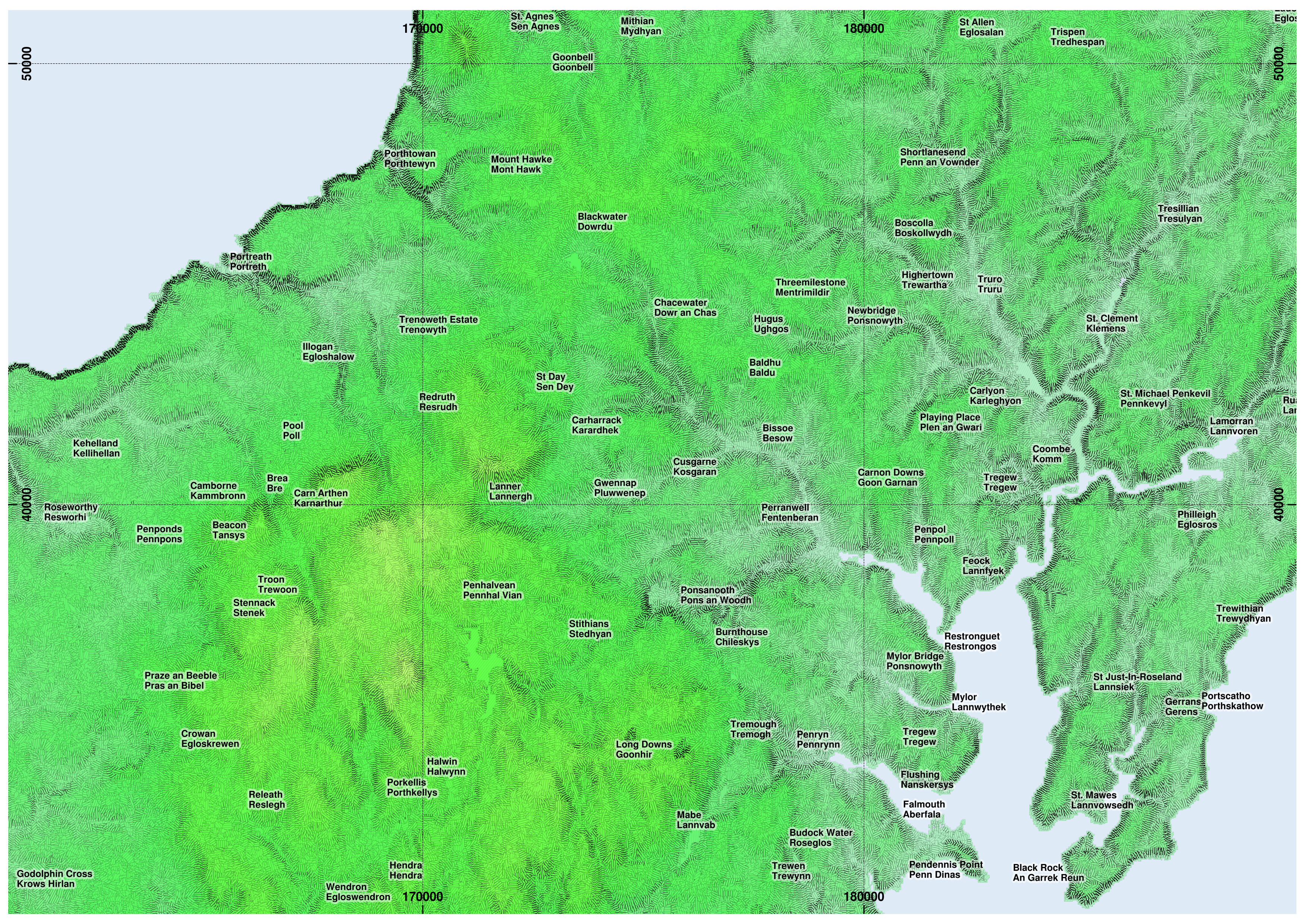
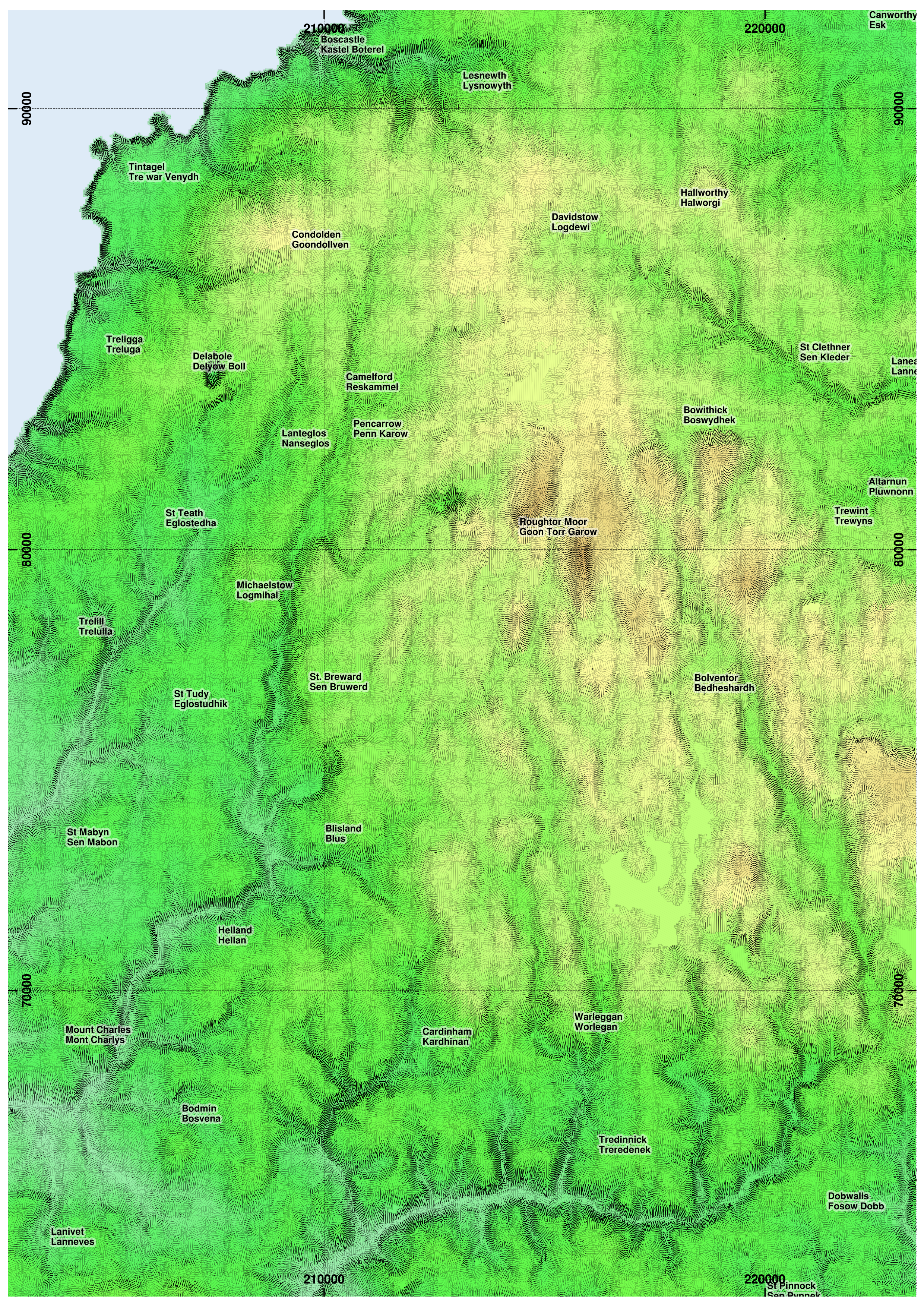
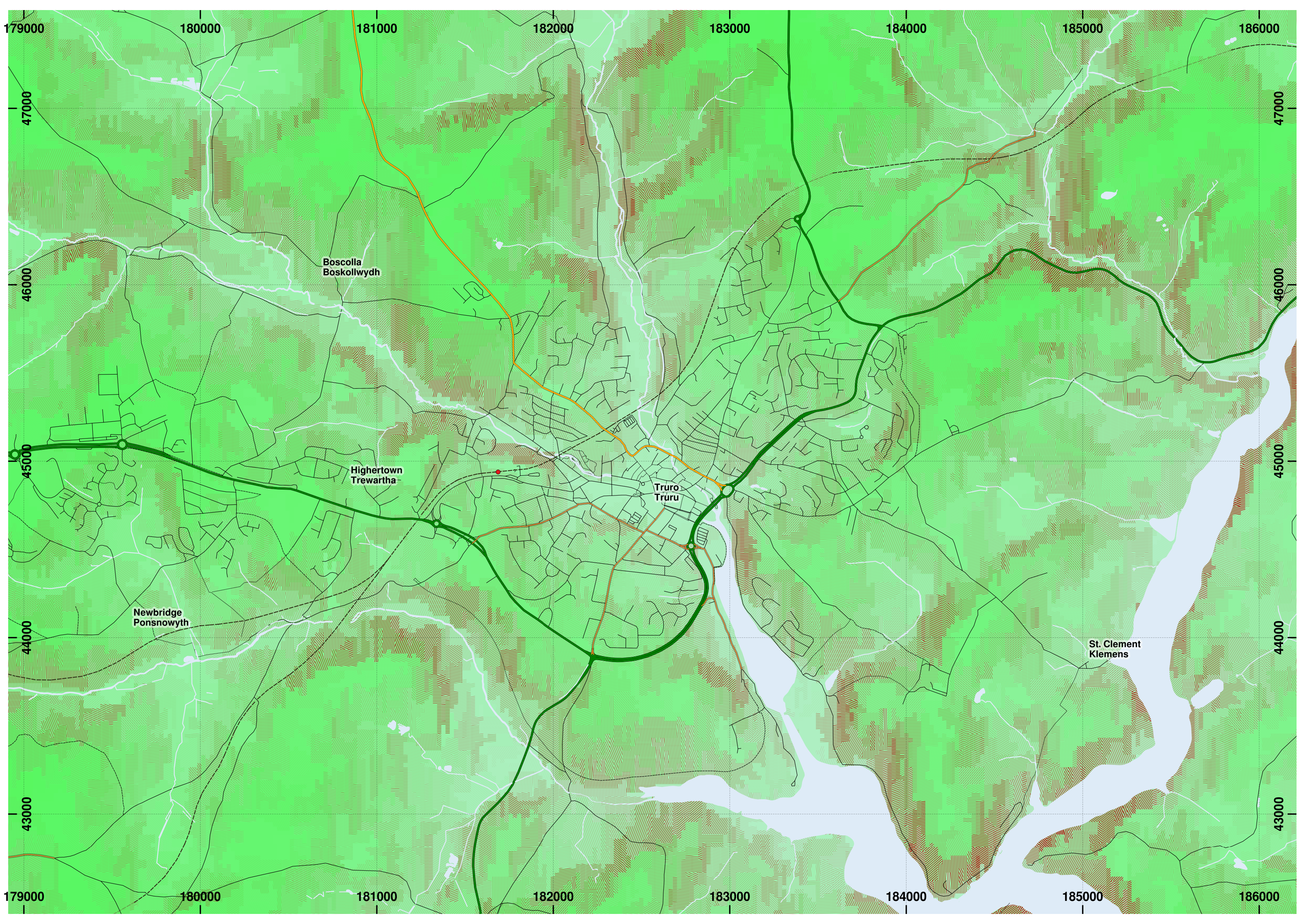
I have put them into QGIS here, and added placename labels for context.

This is the first part of my revisiting this assignment. In future I will also say a little more about the ground control points from the fieldwork and how the results of the classification correspond to what was seen on the ground, and take this a little further than in the assignment report.
What would be really great, is to be able to automatically adjust a ruleset, rather than doing this by hand hard-coding into the scripts.

The Data

Landsat is a programme of Earth observation satellites launched by NASA and operated in cooperation with the US Geological Survey.

They have the capability to take data in several visible light bands, near infrared, short-wave infrared (this is longer wavelength than near-infrared but the common terminology in Earth Observation), and thermal infrared.

Landsat 8 has a slightly different range of wavelengths than Landsat 7, additionally having the 'Coastal' band in band 1 at a slightly shorter wavelength than the Blue band.

The area of study for the assignment was an area of mid-Wales including Aberystwth, and upland areas around Pumlumon.

We were set the images from Landsat 7 from March 2007 and June 2006 to work from, and I additionally used a Landsat 8 image from September 2013. Landsat 7 developer a scan line corrector fault. which resulted in black stripes where no data was collected.

The black no data stripes were ignored, in this classification, my view was to classify based on the data that exists, and perhaps use a nearest neighbour interpolation right at the end after classification if desired.

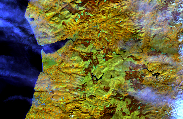
The various Landsat bands allow an overview of land cover types, based on the differing reflectance spectral properties of vegetation of various types, water, and non-vegetated surfaces. Living vegetation is strongly reflectant in the green and near-infrared, with dead vegetation reflecting more strongly at the longer 'short-wave infrared'.

A bank of cloud coincides with the area of study on 6th July 2013

Landsat 7: 9th June 2006, using Bands 3, 2 and 1 (red, green and blue) as RGB.

Landsat 7: 9th June 2006, using Bands 4, 6 and 3 (NIR, SWIR1 and red) as RGB.

Landsat 7: 24th March 2007, using bands 3, 2 and 1 (red, green, blue) as RGB.

Landsat 7: 24th March 2007, using bands 4, 6 and 3 (NIR, SWIR1, red) as RGB.

Landsat 8: 24th September 2013, bands 4, 3 and 2 (red, green, blue) as RGB.

Landsat 8: 24th September 2013, bands 5, 6 and 4 (NIR, SWIR1, red) as RGB.

Classification

A rule based classification was used, inspired broadly speaking by the various Richard Lucas et al. papers: Lucas et al. 2007 Lucas et al. 2011.

Before classification, I first segmented to objects, for which I used the routine in the Python RSGISLib libraries:

The 9th June 2006 image, segmented in RSGISLib using the runShepherdSegmentation method with 120 clusters and a minimum object size of 9 pixels (8100 sq.m), colourized randomly.

In fact I segmented the image three different ways, in the assignment writeup I exclusively used the objects from segmenting the 24th March 2007 Landsat 7 image.
I made a kind of first order seasonal adjustment to the images, based on band averages in areas not classified as cloud or water. It was not entirely successful in creating a consistent classification as seen below.

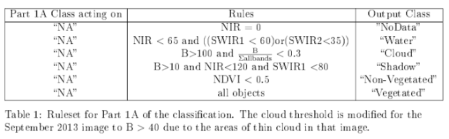
Ruleset

The ruleset I first developed on the March 2007 image because that had areas of cloud and therefore an opportunity to get the cloud masking right first.
There are three stages to the process, first the Level 1A classification that delineates water (by low NIR and SWIR brightness), cloud (by high levels in the blue band), shadow (by thresholds in Blue, NIR, and SWIR1), and non-vegatation (by normalised differential vegatation index (NIR, R)).



After this, in Level 1 split the vegetated areas into woodland, wetland, and heath, and grasslands into unimproved, semi-improved and improved by NDVI.

Level 2 classification splits woodland into broadleaf and coniferous, and wetlands into blanket bog and flush, and the upland vegetation further.

For the other images, I made a first-order seasonal adjustment based on the average band values in non-water and non-cloud objects, effectively attempting to adjust back to the March image. I adjust the NDVI by half of its actual change to avoid overcorrection of the grassland classes, and the Lucas et al. 2011 heath detection index by a manually set value of +3000 in June and +5000 in September.

24th March 2007 segmentation

This was what I used in my report. There is a substantial area under cloud in the SE of the image. I have masked out areas that have No Data in one or both images.

The cloud areas are shown in the SE, generally woodland and water extents are well-recovered. large version

Unfortunately some detail is lost in the uplands, and some areas are spuriously classified as non-vegetated. large version

Modification of the cloud threshold was needed to mask out the extensive areas of thin cloud covering parts of the image. Some spurious water bodies are shown which are in face topographic shadow misclassified as water. large version

6th June 2006 segmentation

 

Again, the summer image does not differentiate the different type of upland vegetation well. The cloud shadow on Borth Bog is misclassified as water. large version

The summer 2006 image is segmented and the spring 2007 data applied, there are some spurious classifications in the cloud shadow areas. large version

The September 2013 data, again showing some spurious areas of water, and some errors around the margins of cloud. large version

24th September 2013 segmentation

I only present the 24th September 2013 data, for this segmentation, due to problems that would be caused by the Landsat 7 no data stripes.

Using the Landsat 8 image for segmentation avoids the stripes of no data, but delimiting the edges of thin cloud is difficult and may result in spurious classifications around the edges. The upland vegetation is not well delineated, with large areas assigned to 'unimproved grassland' or 'Molinia-dominated upland grassland'. large version

The Snows of Olympus, Part II

Here are some more maps from this same area, first focusing on the Acheron Fossae region of the h0037 tile.
I scale the elevation colourization locally:

large version (16MB)

Below, I zoom in on several areas containing several Souness catalogued GLFs, using either colourized elevation, or shading in polygons with ln(K_head), ln(K_ext), and ln(K_ctx) greater than 12, 10 or 10 respectively:

large version

large version of shaded polygons image

 large version

large version

large version

large version

Souness catalogued GLF number 96 merits a closer examination to have a look what is going on with the polygon.

large version

large version

h1210

large version

large version

h1232

large version

large version

h5380

 It looks a little to me like the glacier filled the crater before it receded downwards (large version)

large version